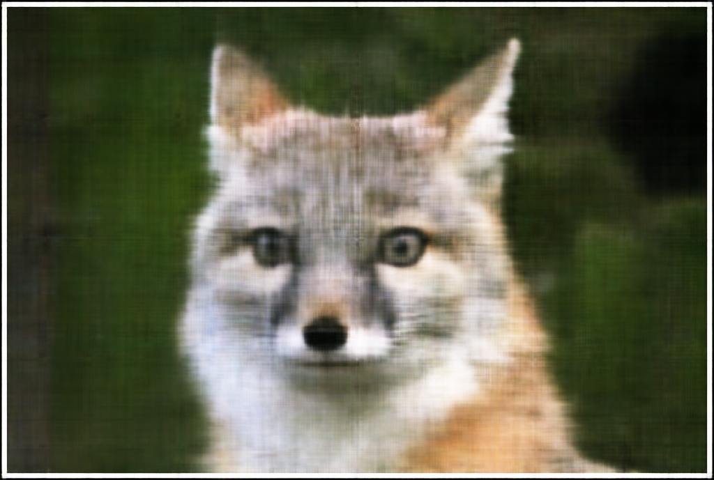

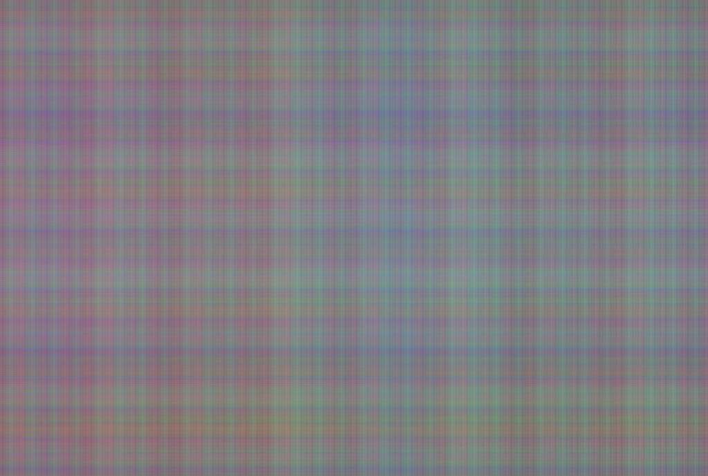
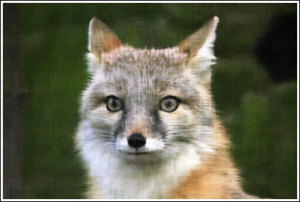
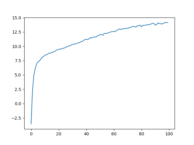
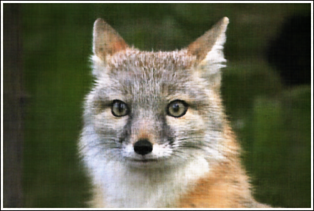
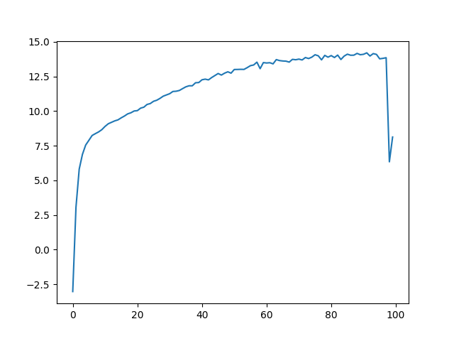
For this, we traing a train a simple MLP to learn the rgb values for a given pixel. First, we implement positional encoding to take the pixel coordinates in the image into a higher dimension representation (by taking the sin and cos values of 2^i * pi * x until L for some value L which we choose to be 10). We also normalize the coordinates to lie from [0, 1] before feeding them into the positonal encoding. The main difference between my implementation and the suggested model is that I used skip layers to allow for deeper models, as well as using a SiLu activation. The first test I did only used 2 hidden layers (so 1 input 2 hidden 1 output).
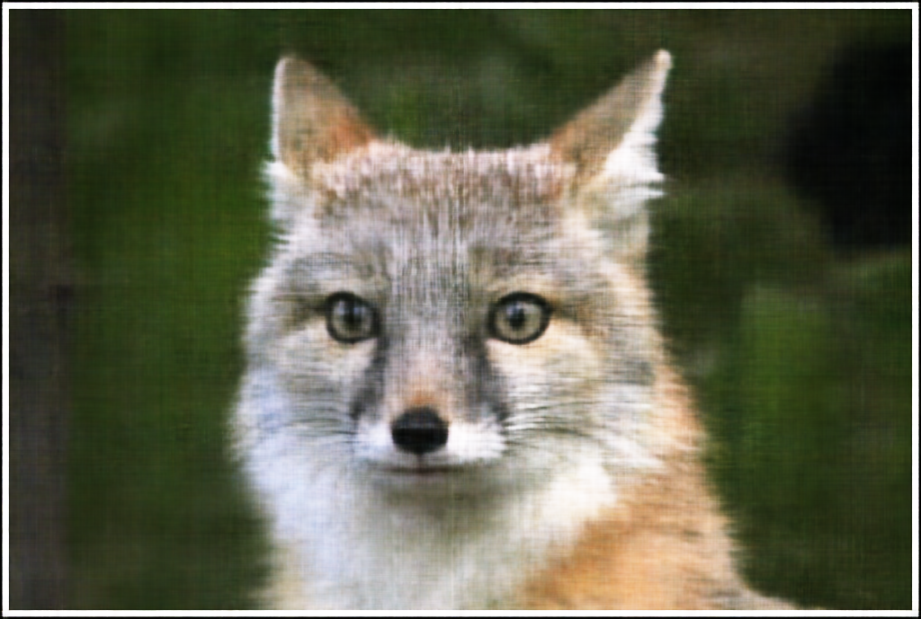
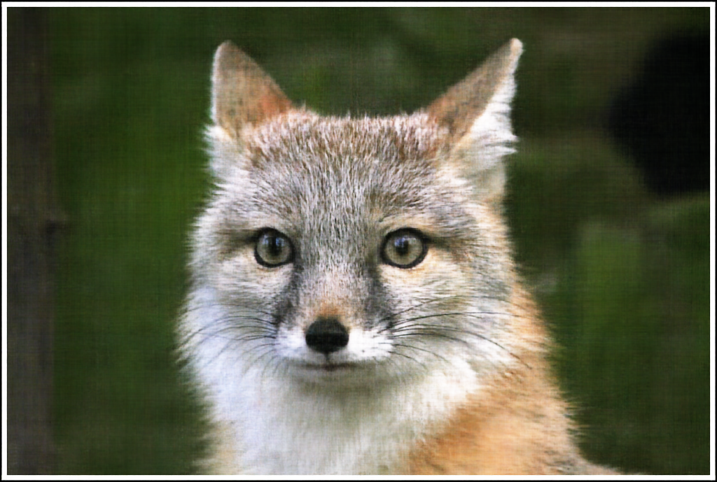
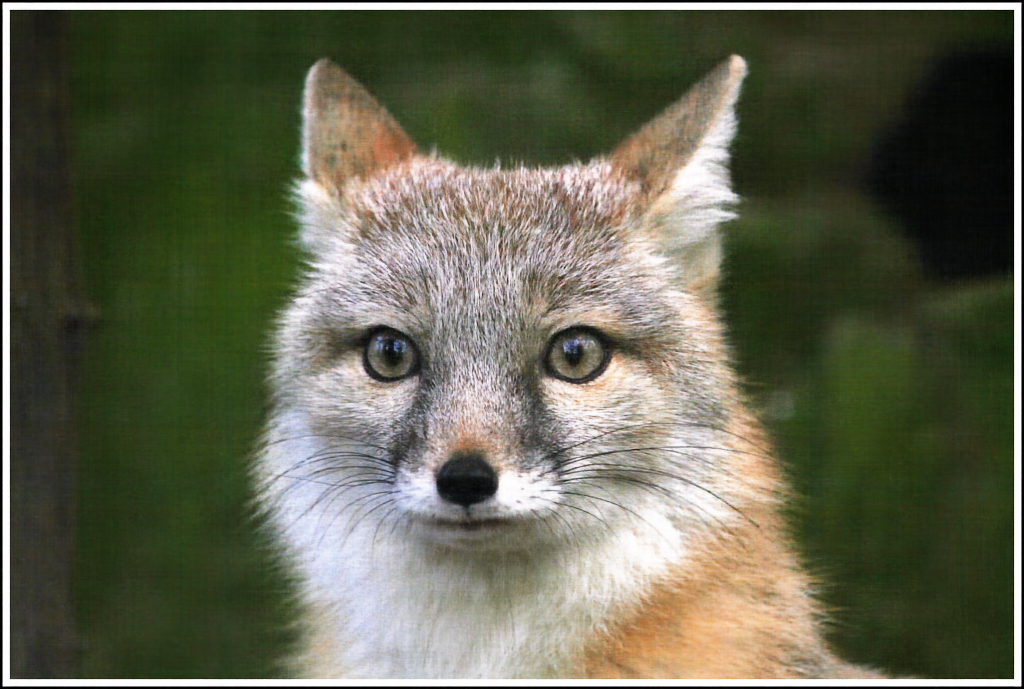
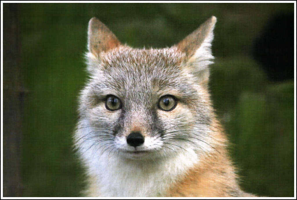
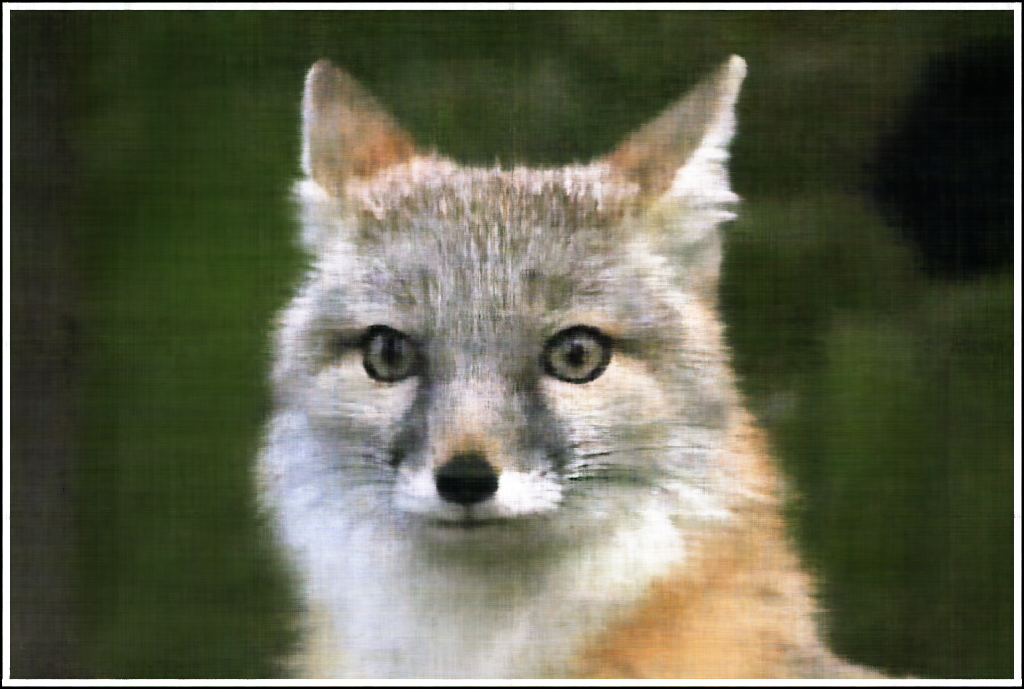
From there, I tested adding more hidden layers, as well as testing increasing the dimension of the encoding L from 10 to 20.
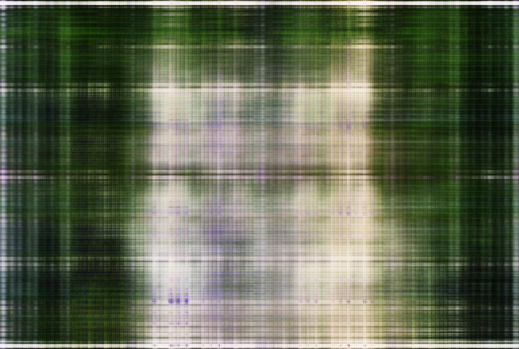
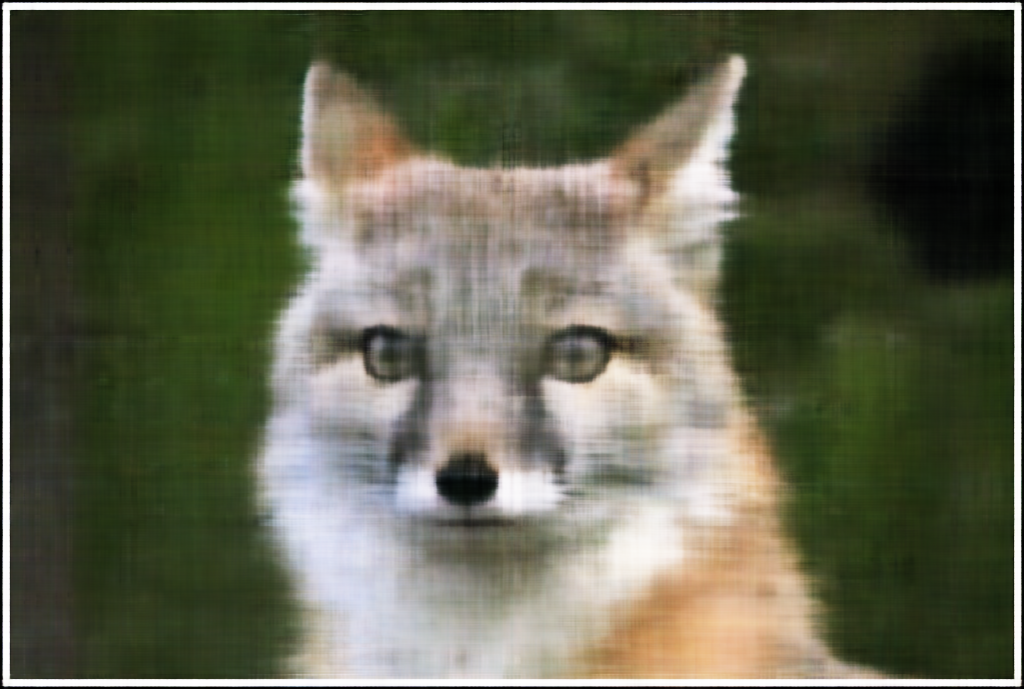
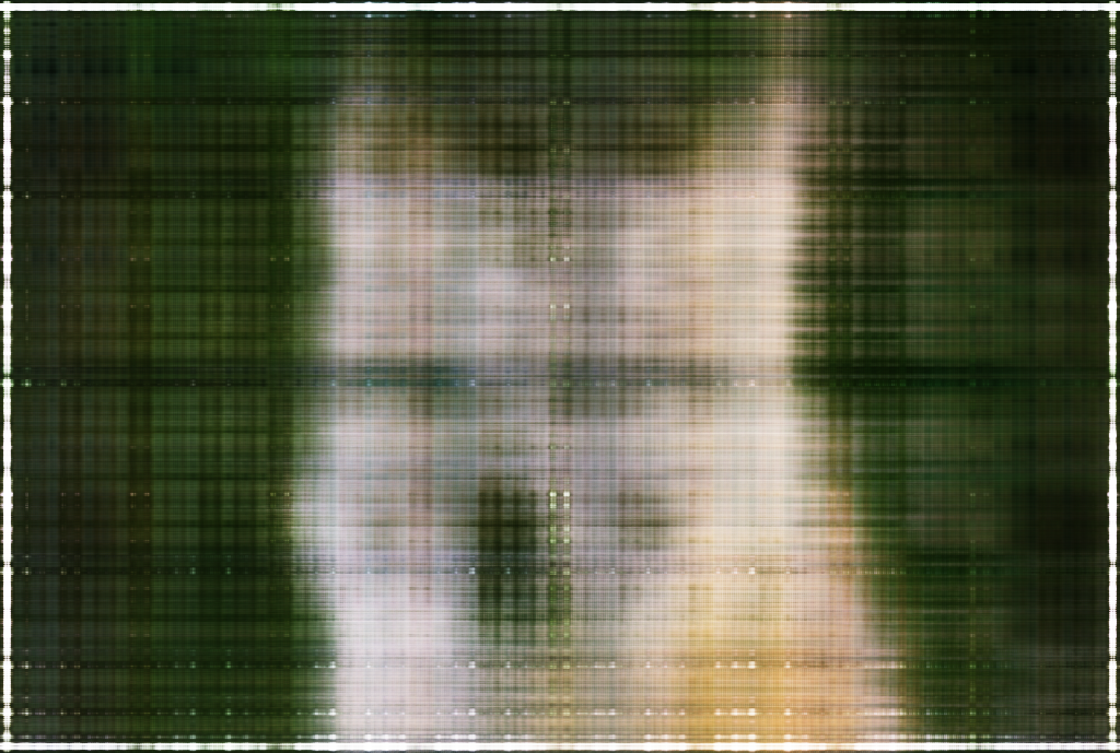
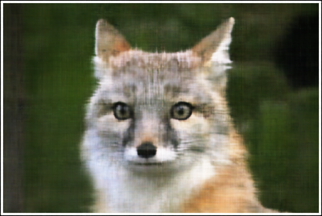
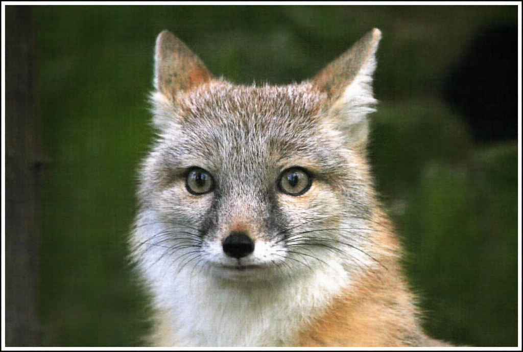
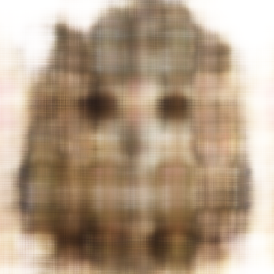
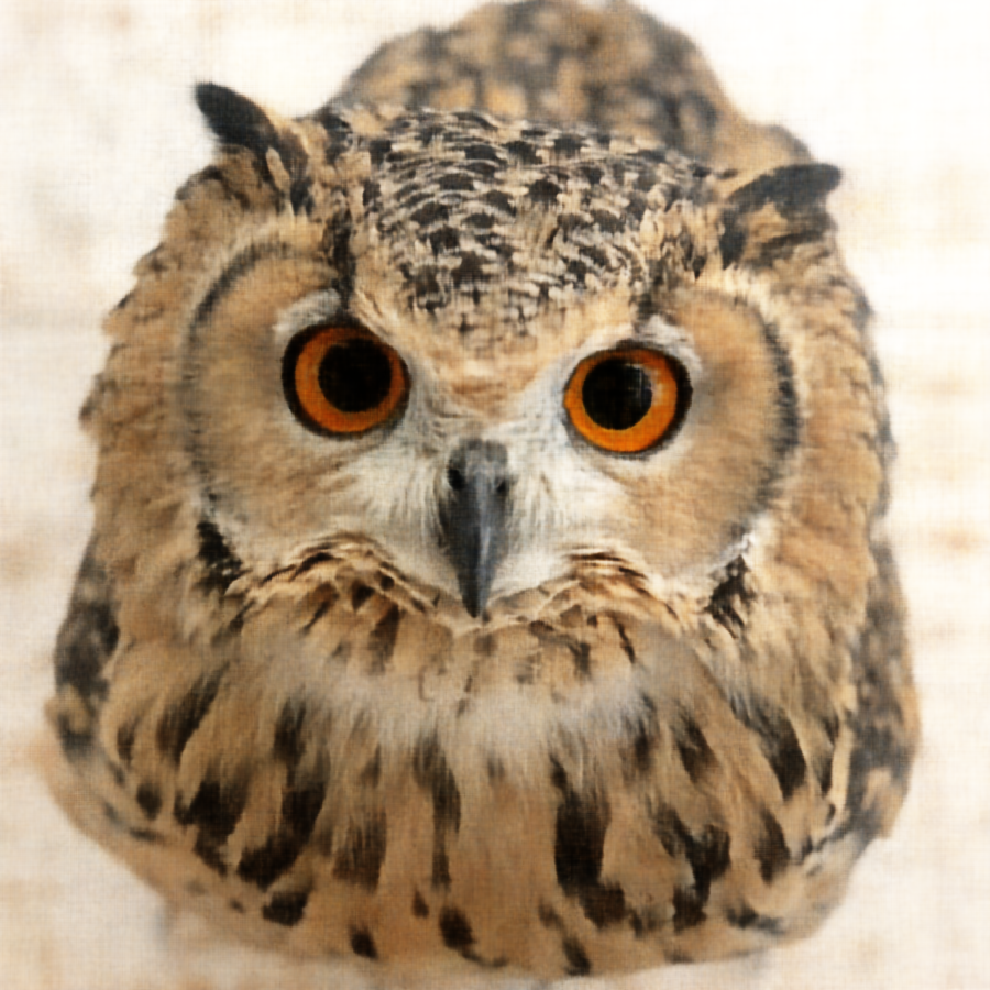
I also did this for one of my own images (an owl). For this I combined both increasing L and the number of hidden layers as they both seemed to improve performance.


Before training a model to fit the neural radiance field, we have to setup the process to handle the images. This involves transforming them
from and to the camera space and world space. We also need to handle the intrinsic matrix to convert between camera coordinates to pixel coordinates.
From there we want get the rays (the origin and ray direction), which we can calculate based on the camera intrinsics, the transformation matrix, and the
pixel coordinates. We also setup a dataset to sample these at random. We also implement sampling points along the rays (somewhat) evenly.
This is done by adding the direction * t (where t is some value from a near and far parameter), and we use 64 t values. We also add a little bit of noise ontop of the
t values in order to prevent overfitting. This gives us the following results when we visualize the setup using viser.
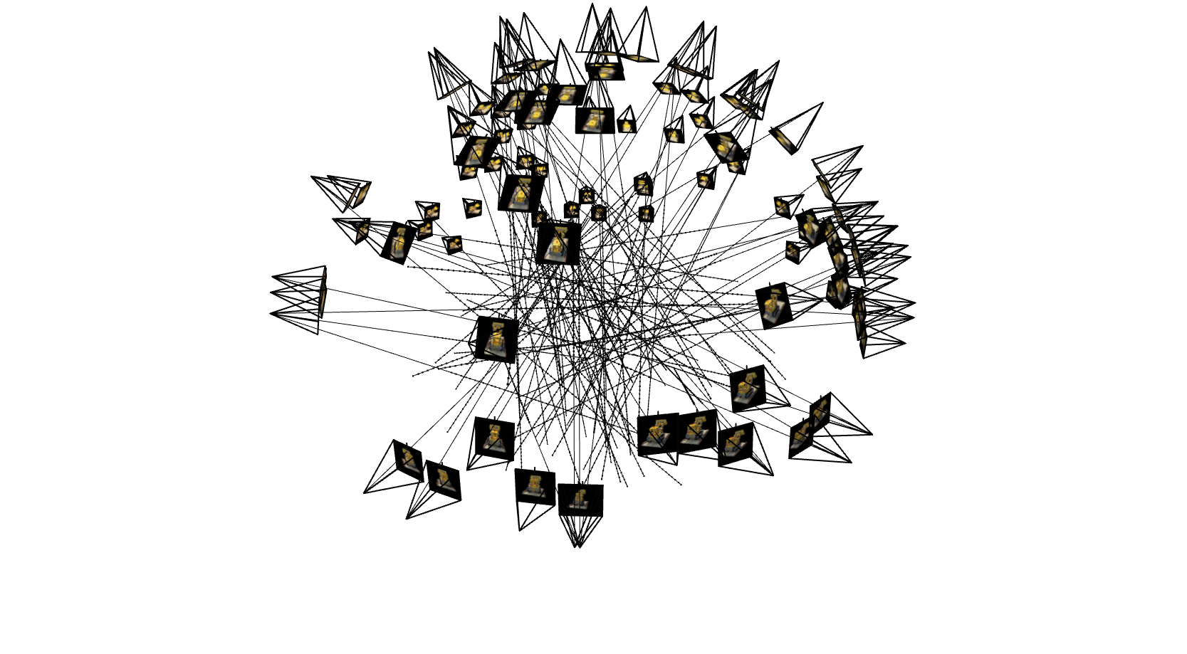
.png)
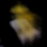
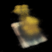
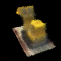
From there, we can start to work on training an MLP to fit the neural radiance field. For our model, we use 12 hidden layers, and similar to
in part 1 we use SiLu and skip connections to allow for this deeper model. We also have to positional encode the ray direction and the
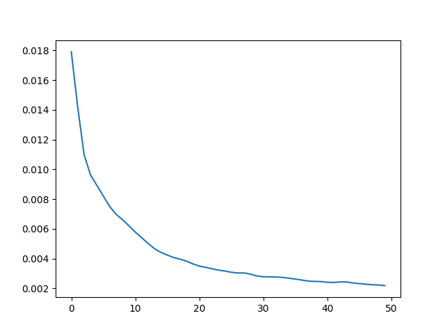
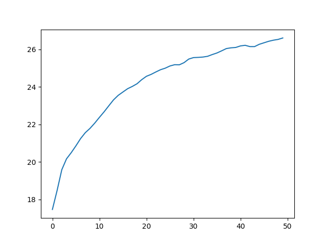
point coordinates. The model then returns a density (or sigma) value and a rgb value. We then use this and a discretized approximation of the volume
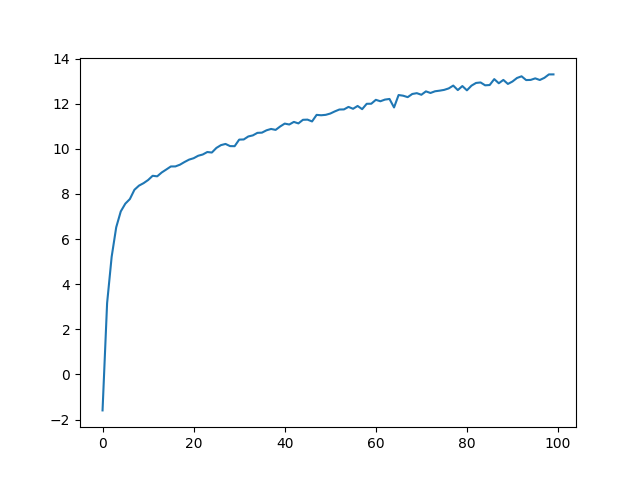
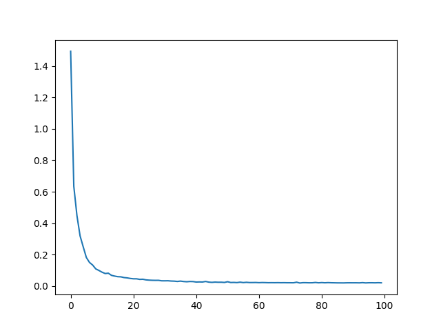
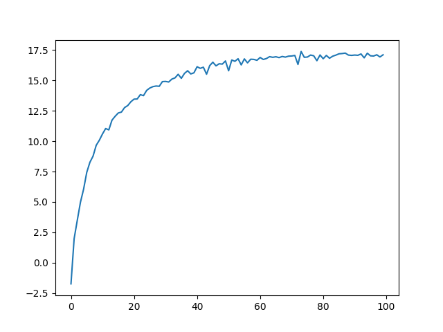
rendering equation in order to produce a pixel color value, which we can use along with the MSE loss to train the model. We train on 50 epochs
of 125 minibatches of size 8000 (so around 5x longer than the staff solution). This took around 30 minutes to train.
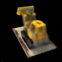
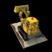
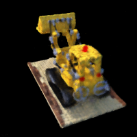
To reconstruct a full image given the transformation matrix, we sample over all u,v pixel coordinates for the image and get the pixel color,
and reconstruct the full image using these colors giving us the example renders below.
I also implemented background rendering. This is done by adding some final background color * the probability of the ray not terminating (which means we can see the background).
I simply did white as it stands out a lot.